
Lab4: Fourier Transform
In the last assignment, we have implemented iDFT to recover discrete signals from frequency domain back to time domain. However, time in the physical world is neither discrete nor finite. In this lab, we will consider Fourier Transform of continuous time signals by combining the sampling theory. In the first part, we will prove that DFT of discrete sampled signals can approximate the Fourier Transform of continuous signals both theoretically and numerically.
Next we will look into the modulation and demodulation of signals. We first prove theorems that shifting a signal in the time domain is equivalent to multiplying by a complex exponential in the frequency domain. To get a better idea of this property, we will again carry out experiments with our voice signals. We will modulate your voice by band-limiting and frequency shifting as well. We will also consider another interesting problem of recovering voice signals separately from a mixed signal.
• Click here to download the assignment.
Computation of Fourier Transform
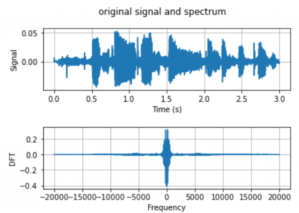
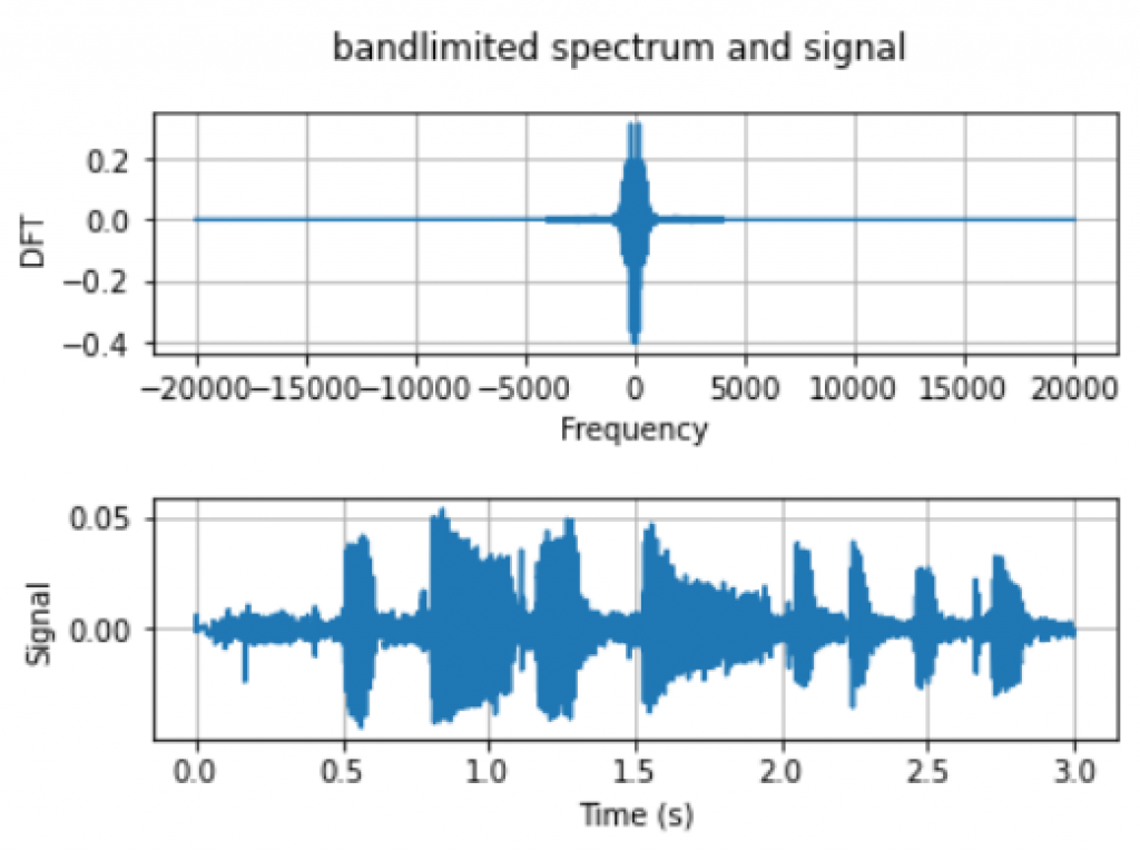
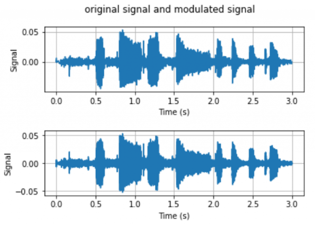
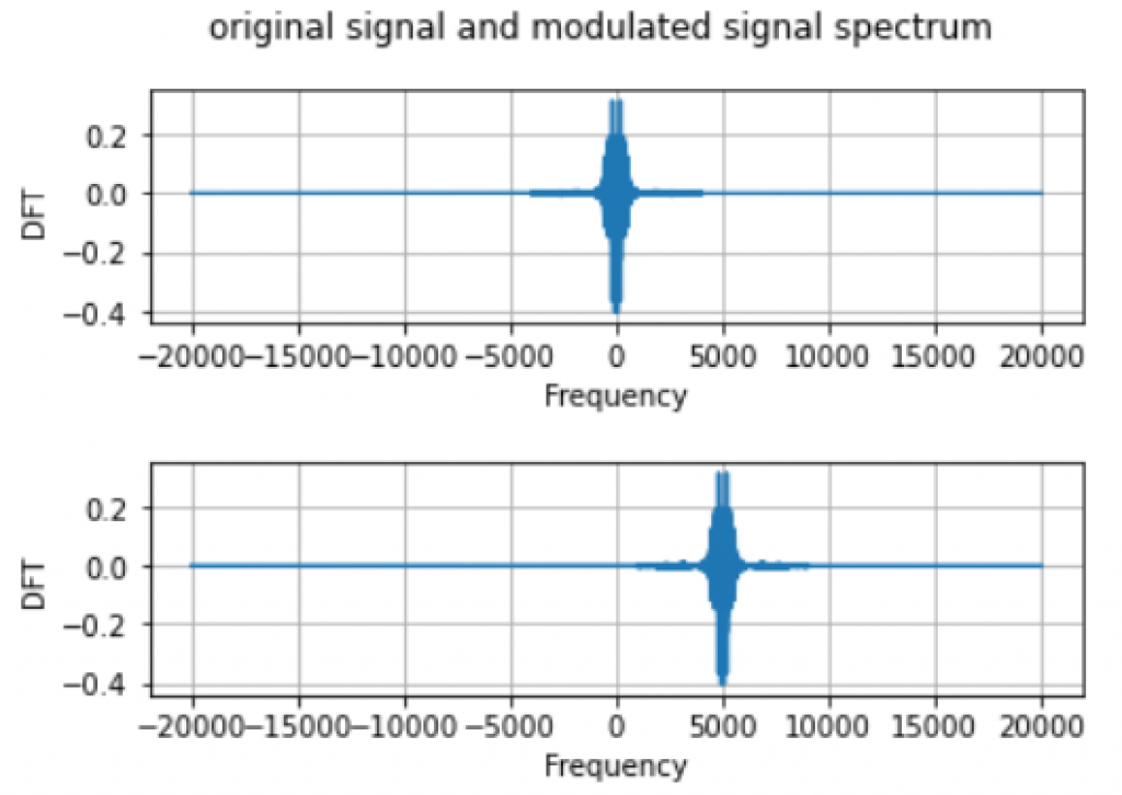
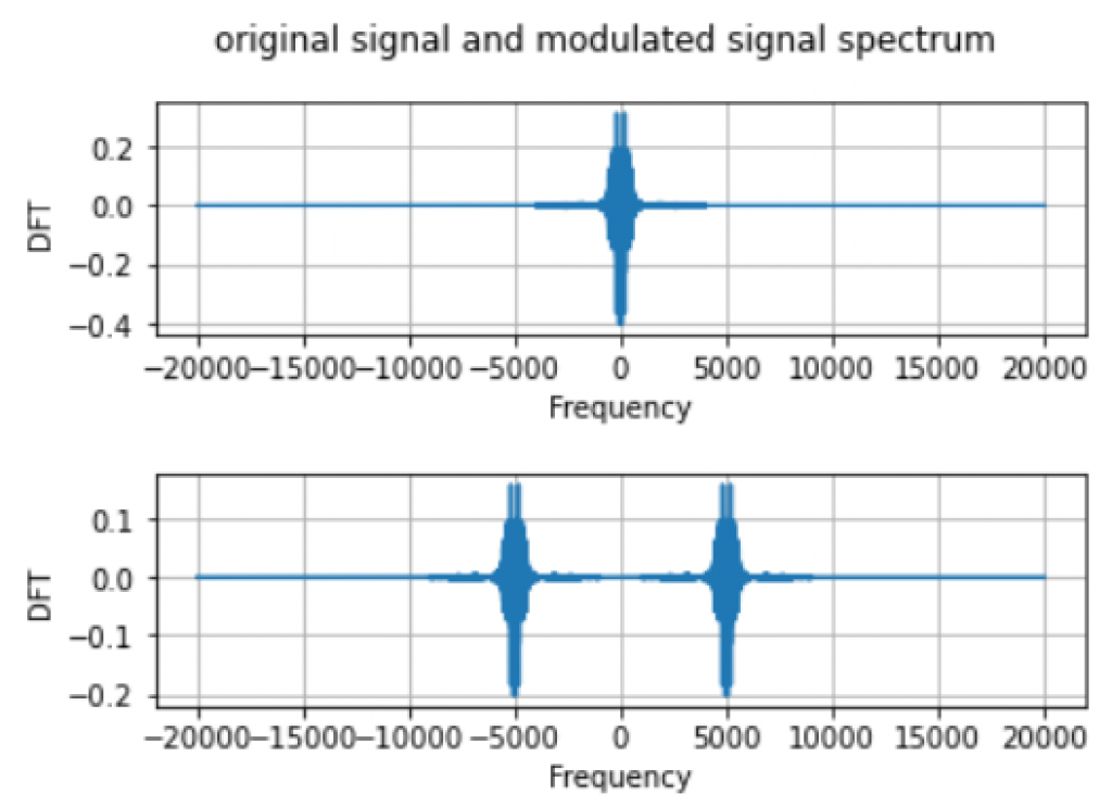
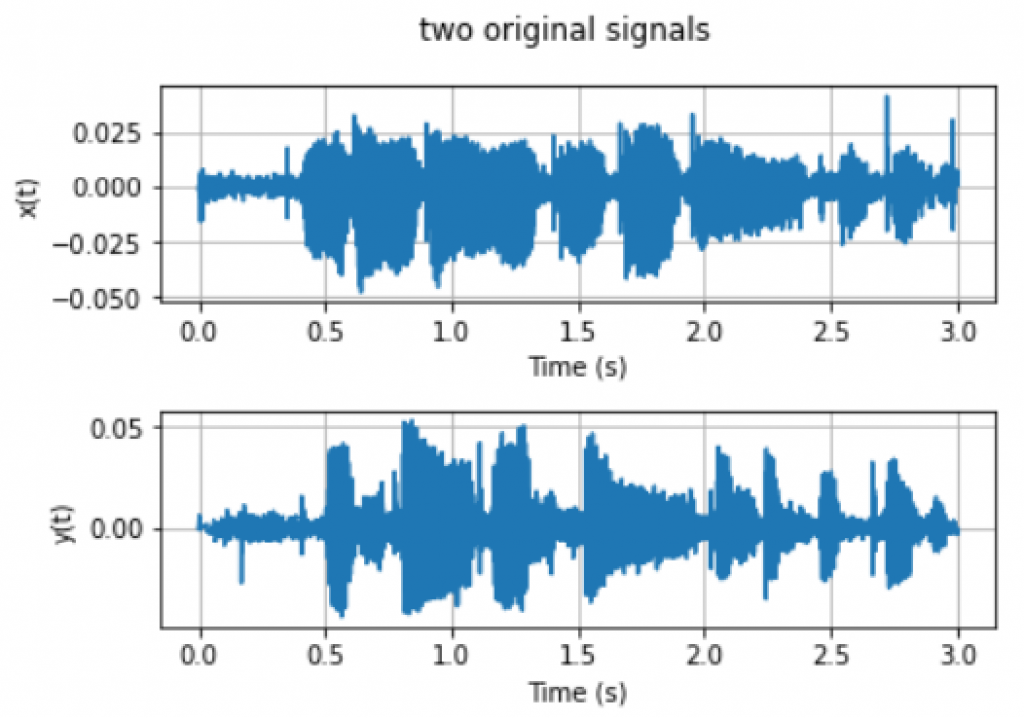
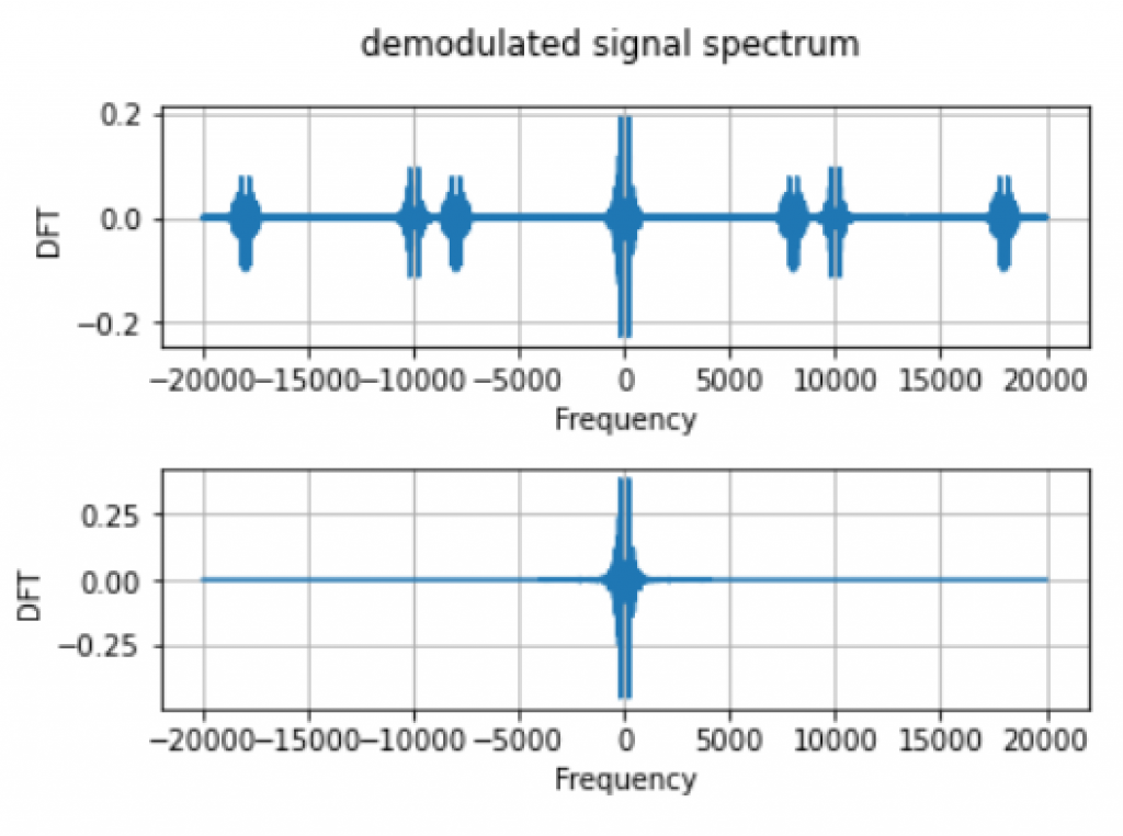
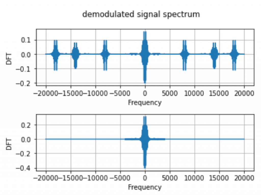
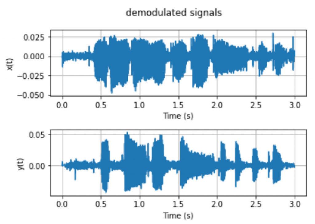
We will first calculate Fourier Transform of specific Gaussian signals with calculus by hand. Fourier Transform of a continuous signal is defined as: \begin{equation}\label{eqn_lab_ft_ft_def} where $x(t)$ is the continuous signal in the time domain and $X(f)$ is its Fourier Transform. Replace $x(t)$ with the given definition of Gaussian pulses when $\mu=0$, we have: \begin{equation} We can solve this integral by completing the squares in the integral term as: \begin{equation}\label{eqn:gau_ft} combined with the given condition that: $\int_{-\infty}^\infty e^{-x^2/(2\sigma^2)}=\sqrt{2\pi} \sigma$. Next we need to verify our derivation with numerical simulations. We need the statement that Discrete Fourier Transform can be seen as approximation of the Fourier Transform. This requires us to utilize $N$ samples of $x$ with a sampling frequency $f_s$ to obtain $N$ samples of $X$ extending from $t=0$ to $t=N/f_s$. As we have done in previous lab assignments, we can use the $\p{dft}$ python class with a sampled discrete Gaussian signal as input. To verify our derived result for the Fourier Transform in \eqref{eqn:gau_ft}, we need to generate frequency signal sequence based on this formula. With the deduction that we have made in class, we know that the relationship between the DFT and FT is: \begin{equation}\label{eqn_lab_ft_approx} Therefore, we can verify our result in \eqref{eqn:gau_ft} by scaling it with $f_s/\sqrt{N}$ and see if the values are the same with DFT in Figure 1. The result in as follows: We can see that Figure 2 is consistent with DFT in Figure 1. This verifies our result and you could also try with other sampling duration and frequency. To derive the Fourier Transform of the Gaussian pulses with generic $\mu$, we could either follow the square completion steps in \eqref{eqn:gau_ft} or use the shifting property, which is shifting a signal in time is equivalent to multiplying it by a complex exponential in the frequency domain. We can get the result in both ways as: \begin{equation} The verification process is the same as above, while we need to consider the shifting term when generating the Gaussian pulse in time domain and the calculated Fourier Transform in frequency domain. One of the important properties of Fourier Transform is that multiplying a signal by a complex exponential results in a shift in the frequency domain. When given signal $x$ and modulated frequency $g$, the modulated signal is defined as: $x_g(t)=e^{j2\pi gt}x(t)$. We denote the Fourier Transform of $x$ as $X=\ccalF(x)$ and Fourier Transform of $x_g$ as $X_g=\ccalF(x_g)$. Based on the definition of Fourier Transform in \eqref{eqn_lab_ft_ft_def}, we have: \begin{equation} Let $u=f-g$, then we have: \begin{equation} combined with the definition of $X(f)=\int_{-\infty}^\infty x(t)e^{-j2\pi ft}dt$. We start by generating a bandlimited signal due to the fact that literally bandlimited signals are hard to find. We again choose to consider voice recordings as we have done in the last lab assignment. First we need to record our voice with $\p{recordsound}$ python class and take DFT of this voice signal with $\p{dft}$ class. We can observe that the frequency components of $f>4kHz$ are very close to zero, which shows our voice signals can be seen as an approximation of bandlimited signals. To be more precise, we need to eliminate the frequency components with frequencies $f>4kHz$, i.e. set $X(f)=0$ with $|f|>4kHz$. We identify the index of frequencies that are within the range $[-4kHz, 4kHz]$ with $\p{where}$ function in $\p{numpy}$ package. By keeping the frequency components unchanged within this range and set those out of the range to zero, we can get the DFT of this bandlimited voice signal. We can use $\p{idft}$ class to transfer back to a voice signal in time domain and play it back. From Figure 5, we can observe that the bandlimited signal is approximately the same as our original signal. The quality of the voice is not reduced if we play back the bandlimited signal. With the definition of the modulated signal $x_g(t)=e^{j2\pi gt}x(t)$, we can take our bandlimited signal generated above and modulate with $g=5kHz$. By taking the DFT of the modulated signal, we can see that the spectrum of modulated signal is now centered at $g=5kHz$, which verifies the modulation property that we have just proved. In a real system we often use the real part to modulate a signal, this leads to the redefinition of modulation at frequency $g$ as: $x_g(t)=\cos(2\pi gt)x(t)$. Recall that with Euler’s formula, a cosine function can be written as a combination of complex exponentials, i.e. \begin{equation} The FT of $x_g$ therefore can be written as: \begin{equation} which leads to the conclusion that: \begin{equation} We can verify this following the steps above. First generate cosine modulated signal by multiplying $\cos(2\pi gt)$ term to the bandlimited signal. Then take the DFT of the modulated signal. From Figure 7, we can see that the spectrum is now centered around $f=\pm 5kHz$ with the magnitude scaled down to the half of the original spectrum. By adding two modulated signals at frequencies $g_1$ and $g_2$, we can get a mixed signal $z(t)=x_{g_1}(t)+y_{g_2(t)}=x(t)\cos(2\pi g_1 t)+y(t) \cos(2\pi g_2 t)$. To recover the signal, we can do demodulation by multiplying the corresponding cosine term and eliminate the frequencies outside the bandwidth defined above, i.e. $4kHz$. As Figure 9 shows, the above spectrum is the DFT of $z_{g_1}(t)=z(t)\cos(2\pi g_1t)$ on the left and $z_{g_2}(t)=z(t)\cos(2\pi g_2 t)$ on the right. After removing the frequency components of frequencies larger than $4kHz$, we have the second row of spectrum in Figure 9. We have now actually recover the spectrum for $x(t)$ and $y(t)$. To recover the signals from frequency domain back to time domain, we use the $\p{idft}$ class and we can also play it back by using the $\p{write}$ function in $\p{scipy.io.wavfile}$. In Figure 10, we can observe that the original signals are recovered. The provided class mentioned in the lab assignment can be downloaded from the folder ESE224_Lab4_provided.zip. This folder contains the following 2 files: The code described here can be downloaded from ESE224_LAB4.Fourier Transform of Gaussian Pulses
{X(f)} := \int_{{-\infty}}^{{\infty}} {x(t)} e^{-j2\pi {f}{t}}{dt},
\end{equation}
X(f) = \int_{{-\infty}}^{{\infty}} e^{- t ^2 / (2\sigma^2)} e^{-j2\pi ft} dt.
\end{equation}
X(f) = e^{-2\pi^2 f^2\sigma^2} \int_{-\infty}^\infty e^{\frac{-(t+2\pi j f \sigma^2)^2}{2\sigma^2}} dt = e^{-2\pi^2 f^2\sigma^2}\sqrt{2\pi}\sigma,
\end{equation}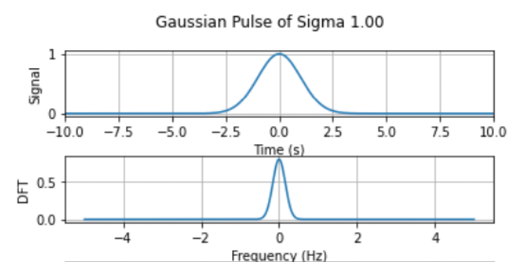
\tdX(k) \approx \frac{f_s}{\sqrt{N}} X(f)= \frac{f_s}{\sqrt{N}} X\left(\frac{k}{N}f_s\right).
\end{equation}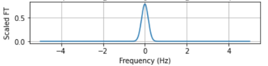
X_\mu(f)=X(f)e^{j2\pi f\mu}=e^{-2\pi^2 f^2\sigma^2+j2\pi f\mu}\sqrt{2\pi}\sigma.
\end{equation}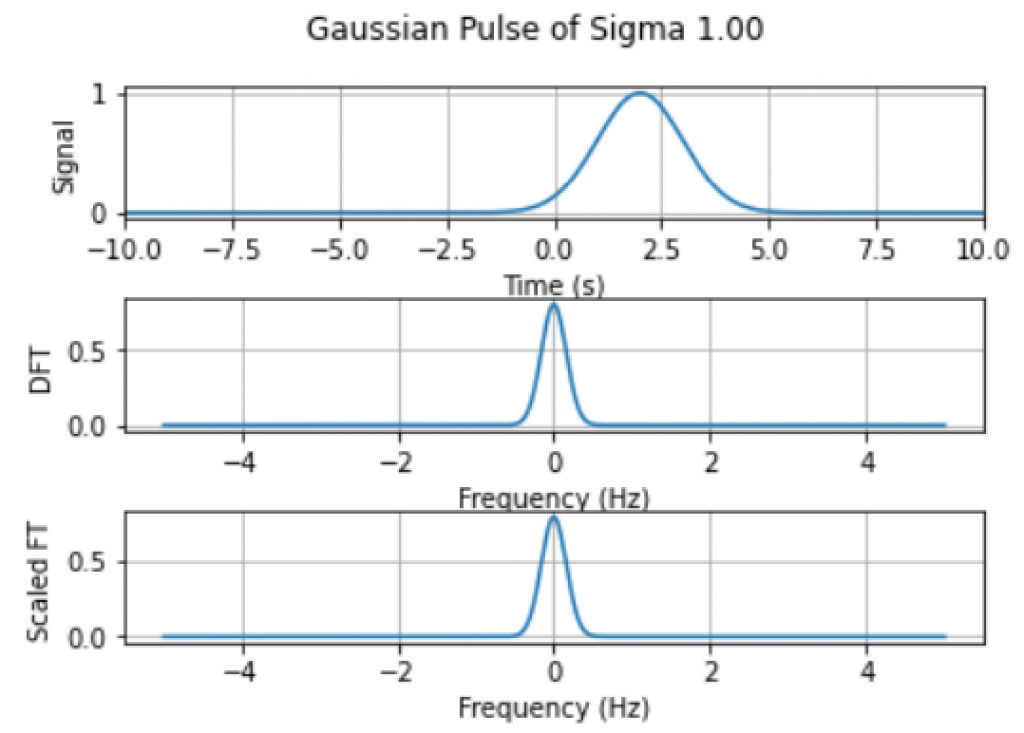
Modulation and Demodulation
X_g=\int_{-\infty}^\infty x_g(t) e^{-j2\pi ft} dt = \int_{-\infty}^\infty x(t) e^{-j2\pi(f-g)t} dt.
\end{equation}
X_g=\int_{-\infty}^\infty x(t) e^{-j2\pi ut}dt = X(u) =X(f-g),
\end{equation}Bandlimited Signals
Exponential Modulation
Cosine Modulation
\cos(2\pi gt)= \frac{1}{2}e^{j2\pi gt} + \frac{1}{2}e^{-j2\pi gt}.
\end{equation}
X_g(f) = \int_{-\infty}^{\infty} \cos(2\pi gt)x(t) e^{-j2\pi ft} dt = \frac{1}{2}\int_{-\infty}^\infty x(t) e^{-j2\pi(f-g)t}dt +\frac{1}{2}\int_{-\infty}^\infty x(t) e^{-j2\pi(f+g)t} dt ,
\end{equation}
X_g(f)=\frac{1}{2}X(f-g) +\frac{1}{2}X(f+g).
\end{equation}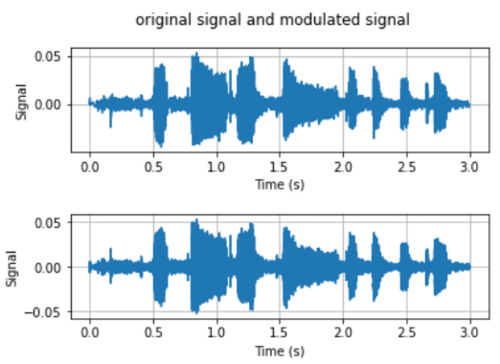
Demodulation
Code links