
Lab3: Inverse Discrete Fourier Transform (iDFT)
We have successfully implemented DFT transforming signals from time domain to frequency domain. However, can we transform these signals back to time domain without losing any information? Why are DFT important for signal and information processing? In this lab, we will learn Inverse Discrete Fourier Transform that recovers the original signal from its counterpart in the frequency domain. We will first prove a theorem that tells a signal can be recovered from its DFT by taking the Inverse DFT, and then code a Inverse DFT class in Python to implement this process.
We will then introduce an important application of DFT and Inverse DFT that is signal reconstruction and compression. We will use DFT and Inverse DFT Python classes to approximate some signals we have seen in previous labs, such as square pulse and triangular pulse, and study how well these approximations are compared with the original signal. We will further deal with the real-world signal – our voice. We will code a Python class that can record and play our own voice, based on which we will implement DFT and Inverse DFT for voice compression and masking. We will end up with an interesting problem allowing you to uncover secret messages from a signal that you may consider normal.
• Click here to download the assignment.
• Due on February 8 by 11:59pm.
Computation of iDFT
In this first part of the lab, we will consider the inverse discrete Fourier transform (iDFT) and its practical implementation. As demonstrated in the lab assignment, the iDFT of the DFT of a signal $\bbx$ recovers the original signal $\bbx$ without loss of information. We begin by proving Theorem 1 that formally states this fact.
Proof of Theorem 1
Given a discrete signal $x:[0,N-1]\to\mbC$, let $X=\ccalF(x):\mbZ\to\mbC$ be the DFT of $x$ and $\tdx=\ccalF^{-1}(X):[0,N-1]\to\mbC$ be the iDFT of $X$. From the definition of the iDFT, we have \begin{align}\label{eqn_lab_idft_idft_def} \tdx(\tdn) = {\frac{1}{\sqrt{N}}} \sum_{{k=0}}^{{N-1}}{X(k)}e^{j2\pi{k}{\tdn}/N} \end{align} Now substituting the definition of the DFT for $X(k)$ in \eqref{eqn_lab_idft_idft_def} yields \begin{align}\label{eqn_lab_idft_dft_def} \tdx(\tdn) = {\frac{1}{\sqrt{N}}} \sum_{{k=0}}^{{N-1}}\Big(\frac{1}{\sqrt{N}} \sum_{{n=0}}^{{N-1}}{x(n)}e^{-j2\pi{k}{n}/N}\Big)e^{j2\pi{k}{\tdn}/N} \end{align} We may exchange the order of the summation, so that we first sum over $k$, and then pull out $x(n)$ since it is independent of $k$, i.e. \begin{align}\label{eqn_proof_theorem1_1} \tdx(\tdn) = \sum_{{n=0}}^{{N-1}} x(n) \Big( \sum_{{k=0}}^{{N-1}} {\frac{1}{\sqrt{N}}} e^{-j2\pi{k}{n}/N} {\frac{1}{\sqrt{N}}} e^{j2\pi{k}{\tdn}/N} \Big) \end{align} Due to the orthonormality proved in 2.4 of Lab 1, we obtain \begin{align}\label{eqn_proof_theorem1_2} \sum_{{k=0}}^{{N-1}} {\frac{1}{\sqrt{N}}} e^{-j2\pi{k}{n}/N} {\frac{1}{\sqrt{N}}} e^{j2\pi{k}{\tdn}/N} = \delta(n – \tdn) \end{align} Therefore, \eqref{eqn_proof_theorem1_1} reduces to \begin{align}\label{eqn_proof_theorem1_3} \tdx(\tdn) = \sum_{{n=0}}^{{N-1}} x(n) \delta(n – \tdn) = x(n) \end{align} with $\tdn = n$ since the only nonnegative term in the sum is when $\tdn = n$.
In the following, We will implement the iDFT in practice and employ it together with the DFT for signal reconstruction and compression on different signals, such as the square pulse, the triangular pulse, etc.
Signal Reconstruction
The original signal $x$ can be recovered exactly by using $N$ summands in the iDFT expression. However, we can also choose to approximate the signal $x$ by the signal $\tilde{x}_K$ which we define by truncating the DFT sum to the first $K$ terms as \begin{align}\label{eq_truncated_reconstruction} \tilde{x}_K(n) := \frac{1}{\sqrt{N}} \left[ X(0)+ \sum_{k=1}^{K} \left( X(k)e^{ j2\pi kn/N} + X(-k)e^{-j2\pi kn/N} \right) \right]. \end{align} As we increase $K$, i.e., adding more DFT coefficients in the truncated sum, we make the approximation closer to the actual signal. Based on the relation between the signal and its DFT we have learned from last lab assignment, we conclude that if we have a signal that varies slowly, a representation with just a few coefficients is sufficient, while for signals that vary faster, we need to add more coefficients to obtain a reasonable approximation.
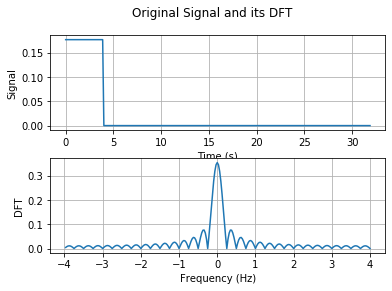
We than first implement the signal reconstruction of a square pulse of duration $T=32$s sampled at a rate $f_s=8$Hz and length $T_0=4$s. According to the definition, the original signal and its DFT are shown in the following figures.
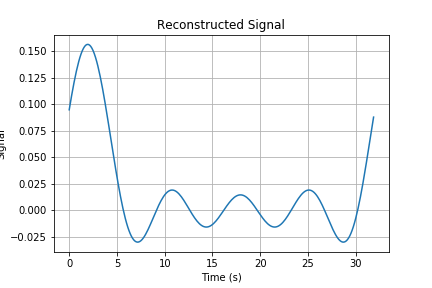
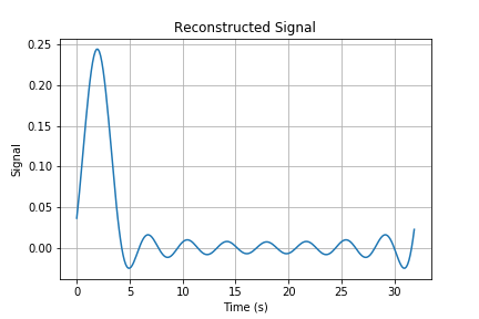
We than reconstruct the signal with the truncated iDFT process. By selecting different truncated parameters $K$, we can reconstruct different approximate signals as follows.
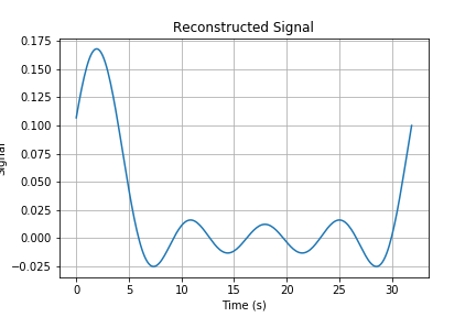
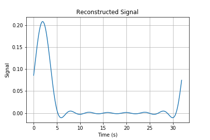
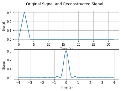
Here we select $K=4$ and $8$ as examples. While in the report, you should try more numbers of $K$ to observe difference between these reconstructed signals. We then implement the signal reconstruction on the second example, the triangular pulse. We show the original signal $x$ and its corresponding DFT coefficients in the following figure.
We then use the truncated $K$ DFT coefficients to reconstruct the signal as $\tilde{x}_K$.
Since the triangular pulse varies more slowly, it should be easier to reconstruct with truncated DFT coefficients. You will find this result more precisely when testing more truncated numbers $K$.
Energy Difference
We study the energy of the difference signal. Denote $\tilde{X}_K$ by the DFT of the reconstructed signal $\tilde{x}_K$, and apply Parseval’s Theorem to have \begin{align}\label{eq_energy_difference_1} \| \rho_K \|^2 = \sum_{n=0}^{N-1} |x(n) – \tilde{x}(n)|^2 = \sum_{k=0}^{N-1} |X(k) – \tilde{X}(k)|^2 = \sum_{k=-N/2+1}^{N/2} |X(k) – \tilde{X}(k)|^2. \end{align} Using the fact that $X(k) – \tilde{X}(k) = 0$ for all $|k| \le |K|$ and $X(k) – \tilde{X}(k) = X(k)$ for all $|k| > |K|$, the energy of the difference signal becomes \begin{align}\label{eq_energy_difference_2} \| \rho_K \|^2 = \sum_{|k|>|K|} |X(k)|^2. \end{align} From above results, the larger $K$ is, the smaller the energy difference is. Therefore, the constructed signal $\tilde{x}_K$ becomes closer to the original signal $x$ if we increase $K$.
Signal Reconstruction with $K$ Largest DFT Coefficients
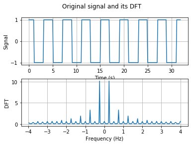
In this subsection, we consider the signal reconstruction with $K$ largest DFT coefficients, which is a different way for signal compression compared with \eqref{eq_truncated_reconstruction}. In this case, we consider the square wave signal of duration $T=32$s sampled at a rate $f_s=8$Hz and frequency $0.25$Hz. We first compute its DFT, find out its largest $K$ DFT coefficients, and reconstruct its approximate signal with iDFT. According to its definition, the original signal and its DFT coefficients are shown in the following figure.
We then reconstruct the signal with $K$ largest DFT coefficients shown as follows.
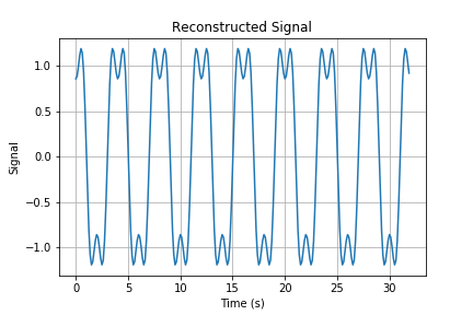
Here we also consider $K=4$ as an example, and you should try different numbers of $K$ to see the difference. We observe that a square wave can be approximated better than a square pulse if you keep the same number of coefficients. This is because the square wave has periodic structure throughout its entire domain, so that we can easily approximate it with a few dominant DFT coefficients. However, the square pulse has a particular structure for the values $0 \le n \le M$ for fixed $M$. Lacking periodic structure, we need more DFT coefficients to effectively reconstruct the signal.
Speech Processing
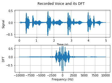
In this subsection, we consider the signal reconstruction for speech signals in practice. We will record our voice, store it as a signal, and employ the DFT combined with the iDFT to perform the signal reconstruction. To begin with, we need to use the toolbox “sounddevice” to record our voice in Python and you should type “pip install sounddevice” in the console for installation. The recorded voice and its DFT is given by
We then use the truncated DFT coefficients for approximate signal reconstruction. We first use the first $K$ DFT coefficients to reconstruct the signal as follows.
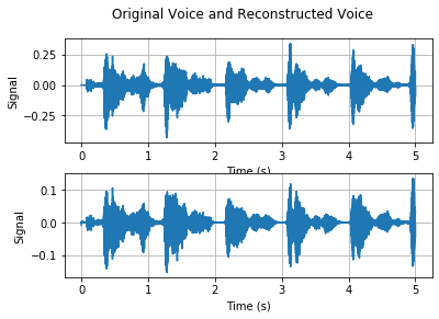
Here, we consider the factor $\gamma=16$, i.e., first $K=6250$ DFT coefficients. You should try different numbers of $K$ in your report to observe the difference. We then consider another strategy for signal reconstruction. That is, we use the largest $K/2$ DFT coefficients as shown below.
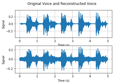
You should do both signal reconstruction strategies with different numbers $K$. By comparing these results, we observe that the signal reconstruction with largest $K/2$ DFT coefficients typically works better than the signal reconstruction with first $K$ coefficients, while we note that this result also depends on the number $K$.
Voice Masking
You can reconstruct your voice signal by different truncation strategies. In particular, you can manipulate the spectrum as you prefer to reconstruct different approximate signals. One possible strategy is that we only store the DFT coefficient whose magnitude is smaller than a preset threshold $\alpha$, which is shown in the following figure.
We consider the threshold $\alpha=0.25$. In your report, you can try different strategies for signal reconstruction with your creativity and observe your results.
MP3 Compressor
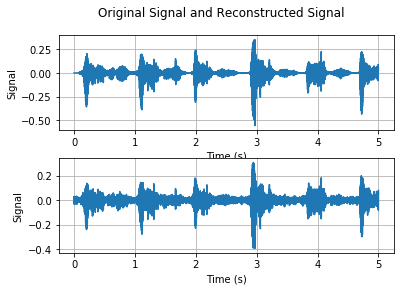
Lastly, we consider a better voice compression strategy that divides your speech in chunks of 100ms, and compresses each of the chunks by a given factor $\gamma$. This is also a rudimentary MP3 compressor, and we show the original signal and the reconstructed signal as follows.
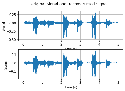
We consider the factor $\gamma=16$ as an example. We may observe that the MP3 compressor recovers the original signal better. In your report, you should try different factors $\gamma$ and try to push $\gamma$ the largest possible compression factor.
Code Links
The provided code mentioned in the lab assignment can be downloaded from the folder ESE224_Lab3_providedcode.zip. This file contains the provided python classes, but note that the file itself does not perform any computation.
- The class $\p{recordsound()}$ is defined in this file to record voice signals.
- The class $\p{idft()}$ implements the inverse discrete Fourier transform in $2$ different ways.
- The class $\p{tripulse()}$ generates the triangular pulse signal.
- The class $\p{sqpulse()}$ generates the square pulse signal.
The code described here can be downloaded from the folder ESE224_Lab3_Code_Solution.zip. This folder contains the following 2 files:
- $\p{discrete\_signal.py}$: This file defines the functions that generates different types discrete signals.
- $\p{ESE224\_Lab3\_Main.py}$: This file defines the functions that we used to solve the problems in the lab assignment, instantiating objects when necessary. This is also where the plots and the voice record files are created.