DFTs are based on complex exponentials, and as expected DCTs will be based on 2-D discrete cosines. This allows us to still represent a signal as a sum of oscillations, but avoids the border discontinuities that we saw happen with DFTs. We first introduce the two-dimensional discrete cosine $C_{k,l}(m,n)$ of frequencies $k,l$, defined as:

\begin{equation} C_{k,l}(m,n) = \cos\left( \frac{k\pi}{2M}(2m+1) \right) \cos\left( \frac{l\pi}{2N}(2n+1)\right). \end{equation}

The two-dimensional DCT of a signal x is then given by substituting $\bbC_{kl, MN}$ into the expression for the two-dimensional DFT. The DCT will be given by:

\begin{align}
X_C(k,l) &= \frac{2}{\sqrt{MN}} \sum_{m=0}^{M-1} \sum_{n=0}^{N-1} x(m,n)c_1 c_2 \cos\left( \frac{k\pi}{2M}(2m+1) \right) \cos\left( \frac{l\pi}{2N}(2n+1)\right)\\
& = \frac{2}{\sqrt{MN}} \langle \bbx, \bbC_{kl,MN}\rangle,
\end{align}

where $c_1=1/\sqrt{2}$ for $k=0$ and $c_1=1$ for $k=1, 2\dots M-1$, $c_2=1/\sqrt{2}$ for $l=0$ and $c_2=1$ for $l=1, 2 \dots N-1$. Similarly to the DFT case, the expression for the DCT can be seen as inner product of a signal with a discrete cosine. Therefore we can take use of the $\p{inner\_prod\_2D}$ python class that we have used in the last lab and replace the complex exponential matrix with the discrete cosine matrix that we have just defined. To generate the cosine matrix of frequencies $k,l$, we can use $\p{np.matmul}$ function. We can use a nested for loop to calculate cosine matrix for each $k,l$ pair.

When the signal dimension is very large, it takes a very long time to compute the nested for loop structure. We therefore recommend the built-in $\p{dct}$ function in the $\p{scipy.fft}$ package to accelerate the process.

Image Compression

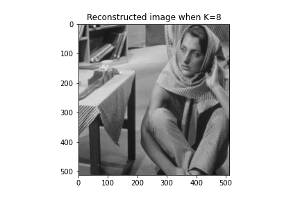
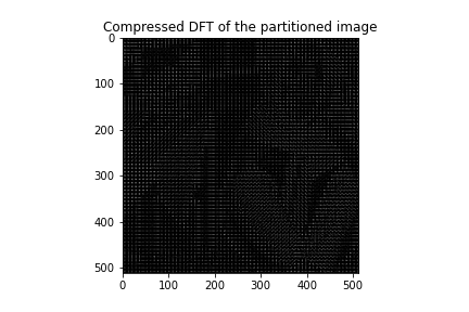
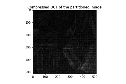
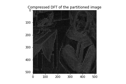
Similar to the audio compression scheme that we have carried out in Lab 3, we can write a python class to partition the input image into $8\times 8$ patches. By keeping the $K$ largest DFT or DCT coefficients in each patch, we can compress the image in this way.

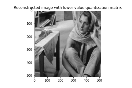
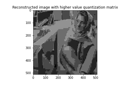
Quantization

This part asks us to implement a basic version of the JPEG compression scheme. That scheme consists, roughly speaking, of partitioning the image into patches, performing the discrete cosine transform on each patch, and finally quantizing (i.e. rounding) the corresponding DCT coefficients. That is, this compression scheme would consist of the following steps:

1. Extract an $8\times 8$ block of the image. Recall that our image signal corresponds to an $N\times N$ matrix. That is what we would obtain after importing an image with $\p{matplotlib.image.imread}$ function in Python. Thus, to create the blocks or patches, we can think of each block as a ’submatrix’ $x_{ij}$, with $(i, j)$ the position of the first pixel of that block.
   
2. Compute the DCT of each $8\times 8$ block. Then we need to store that resulting signal in $X_{ij}$. Since we are working here with two-dimensional signals, $X_{ij}$ will be another block of $8\times 8$ elements $X_{ij} (k, l), k, l \in \{1, . . . , 8\}$.
   
3. After computing the DCT of each block, we now have access to the frequency components of the signal. We will then quantize the DCT coefficients, that is, we will compute:
   \begin{equation} \hat{X}_{ij}(k, l) = \text{round} \left[ \frac{X_{ij}(k, l)}{Q(k,l)} \right] \end{equation}
   where $Q(k, l)$ is a quantization coefficient. That quantization coefficient is used to control how much that particular $(k, l)$ frequency is quantized. To each of the (DCT) patches $X_{ij}$, we will apply a standard $8\times 8$ JPEG quantization matrix $Q_L$. We need to define this matrix as given in the lab assignment. We can use $\p{np.matmul}$ to carry out the element-wise division.
   

Reconstruction

In part 1.4 we are asked to implement the inverse operation to the compressed DCT in part 1.2 as well as the quantized DCT in part 1.3. Given an image that was compressed according the one discussed in question 1.2 or the JPEG compression scheme, we need to reconstruct the image. That would amount to the following steps:

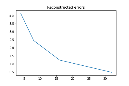
1. Extract an $8\times 8$ block of the compressed DCT matrix. Dequantize the coefficients if we want to reconstruct a JPEG compressed image. This means to multiply the quantization matrix element-wise but without the round calculation.
   
2. Compute the inverse DCT of each patch. To make this process faster, we again make use of the built-in function $\p{scipy.fft.idct}$.
   
3. Stitch the patches together and calculate the reconstruction error according to the equation:
   \begin{equation} \rho = \|\bbx -\hat \bbx\|
   \end{equation}
   

From Fig 3, we can observe that the reconstruction error decreases as the number of reserved frequency components $K$ increases. In Fig 4, when using a quantization matrix with lower value, the reconstruction is better than standard quantization matrix if we look into the reconstruction error. Notice that we need to make sure there is no zero entry in the quantization matrix. When using a higher value quantization matrix, the reconstruction becomes worse for it eliminates more frequency components.

Code links