
Lab 12: Signal Processing on Graphs
The goal of this lab is to introduce Graph Signal Processing. In previous weeks, we have focused our attention on discrete time signal processing, image processing, and principal component analysis (PCA). These three seemingly unrelated areas can be thought of as the study of signals on particular graphs: a directed cycle, a lattice and a covariance graph. Thus, the theory of signal processing for graphs can be conceived as a unifying theory which develops tools for more general graph domains and, when particularized for the mentioned graphs, recovers some of the existing results.
• Click here to download the assignment.
• Click here to download the data for the assignment.
Connection with traditional Signal Processing
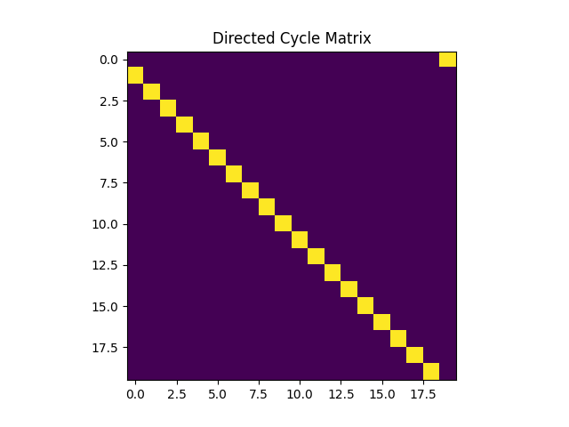
In the first part of this lab, we will generate a directed cycle graph which we will denote $A_{dc}$. We are asked to write a class that takes as an input the number of nodes $N$ as outputs the adjacency matrix of the unweighted directed cycle graph. The code can be implemented as follows,
class matrix:
    def __init__(self,N):
        self.N=N

class directCycle(matrix):
    def __init__(self,N):
        super().__init__(N)
        self.A=np.tril(np.ones((self.N,self.N)),-1)-np.tril(np.ones((self.N,self.N)),-2)
        self.A[0,self.N-1] = 1
The directed cycle graph can be shown using the function $\p{imshow}$ as follows,
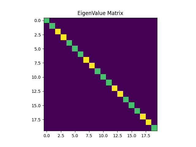
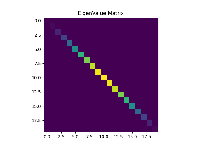
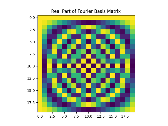
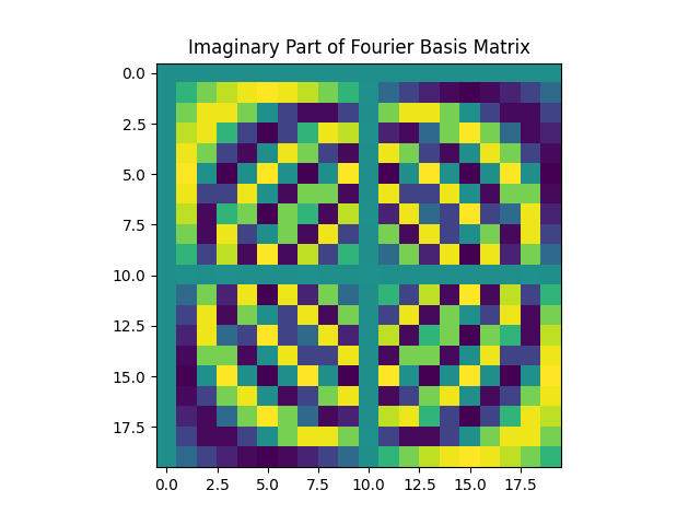
Next, we are required to consider two graph shift operators (GSO) $S_1=A_{dc}$, and $S_2=Laplacian(A_{dc}+A_{dc}^T)$. Note that $S_2$ is indeed a symmetric GSO. We then consider the Discrete Fourier basis $F$, and we show the result of $\Lambda_i=F S_i F^H$, with $i=\{1,2\}$. The structure of both $\Lambda_1$, and $\Lambda_2$ should be the same, they should both be diagonal matrices. What this is telling us is that the Hermitian of the Fourier matrix $F^H$ are the eigenvectors of $S$. Besides, obtaining a diagonal matrix confirms that the DFT and the GFT are equivalent in this case. Notice that the DFT of a signal is computed as $Fx$ and the GFT as $V^Hx$. Plus, we know that $V = F^H$ and the result follows. All the same conclusions hold for both $S_1$, and $S_2$.
The Graph Frequency Domain
In this part of the lab we will write a python class that computes the graph fourier transform. To do so, we will have as an input, the GSO, and we will write 3 methods. The first one is $\p{computeGFT}$ which given a signal $x$ computes the graph fourier transform. The second one is $\p{computeiGFT}$ which computes the inverse graph fourier transform of a given graph signal $xt$. And finally, $\p{computeTotalVariation}$ which calculates the total variation of a signal $x$.
class GFT:
    def __init__(self,S):
        self.S=S
        [self.eigs,self.V]=np.linalg.eig(S)
        self.V=self.V[:,np.argsort(self.eigs)]
        self.eigs=np.sort(self.eigs)
        self.Lambda=np.diag(self.eigs)

    def computeGFT(self,x,k=None):
        xt=np.conj(self.V.T) @ x
        if k==None:
            return xt
        else:
            xtk = np.zeros_like(xt)
            xtk[np.argsort(np.abs(xt[:, 0]))[-k:], 0] = xt[np.argsort(np.abs(xt[:, 0]))[-k:], 0]
            return xtk

    def computeiGFT(self,xt, k=None):
        if k==None:
            return self.V@xt
        else:
            return self.V[:,np.argsort(np.abs(xt[:,0]))[-k:]]@xt[np.argsort(np.abs(xt[:,0]))[-k:],0]

    def computeTotalVariation(self,x):
        return x.T@(self.S)@x
Using the data provided in this lab, we can verify that the graph $A$ has one connected component by evaluating the multiplicity of the eigenvalue $0$. Recall that the multiplicity of the eigenvalue $0$ is the same as the number of connected components of the graph, which is this case is equal to one. If we plot the $3$ signal on the graph, it yields,
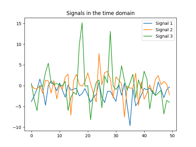
Analogous to plotting songs in the time domain (cf. labs 2 and 3), not much can be said from the figures. In particular, if we need to answer the question, which signal varies faster on the graph, we wouldn’t be able to. However, we can resort to the GFT to extract information about signals. If we take a look at the GFT of the same $3$ signals, it is clear that signal $3$ varies faster in the graph. Note that signal $3$ is expressed using higher-order frequencies of the GFT.
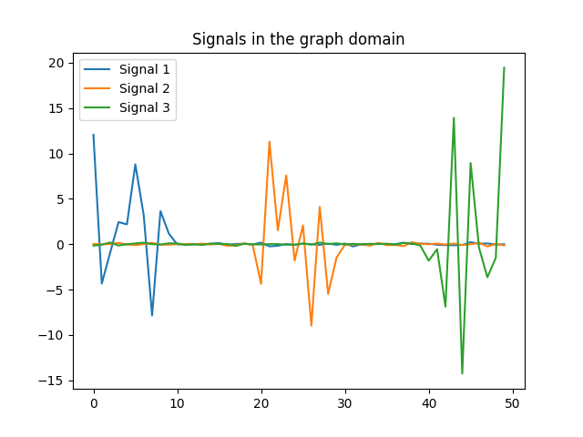
We are also required to obtain the total variation of each signal on the graph. Recall, that we can obtain the total variation of a signal on a graph, by computing the quadratic form on the Laplacian of the graph, namely $TV_{G}(x)=x^T L X$. The values of the total variation are expressed in the following table,
| Signal | Total Variation |
|---|---|
| $x_1$ | $241.8$ |
| $x_2$ | $1385.6$ |
| $x_3$ | $8761.3$ |
If we compare the results of table 1 with figure 4, we can conclude that they are consistent. Signal $x_3$ has the largest total variation in table 1, and in figure 4 we can see that its GFT decomposition, takes values on larger frequencies.
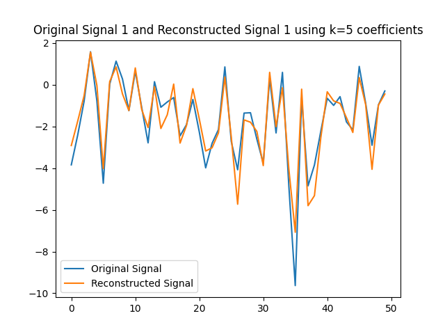
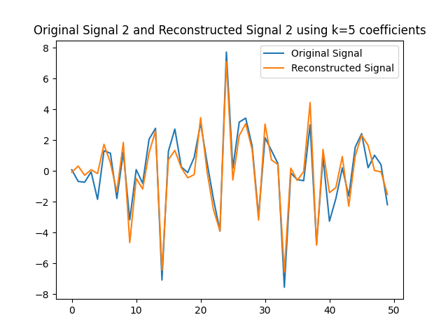
We can use the $k=5$ largest coefficients to reconstruct the signal. By doing so we will be able to obtain a reconstructed signal that resembles the original signal yet it uses $k=5$ instead of $50$ coefficients on the GFT. In this part of the lab, we will obtain the GFT and keep only the $k=5$ coefficients with the largest absolute value. In the following figures, we obtain the reconstructed signals and GFTs of the signals, and of their compressed counterpart.
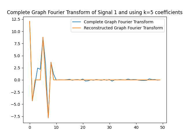
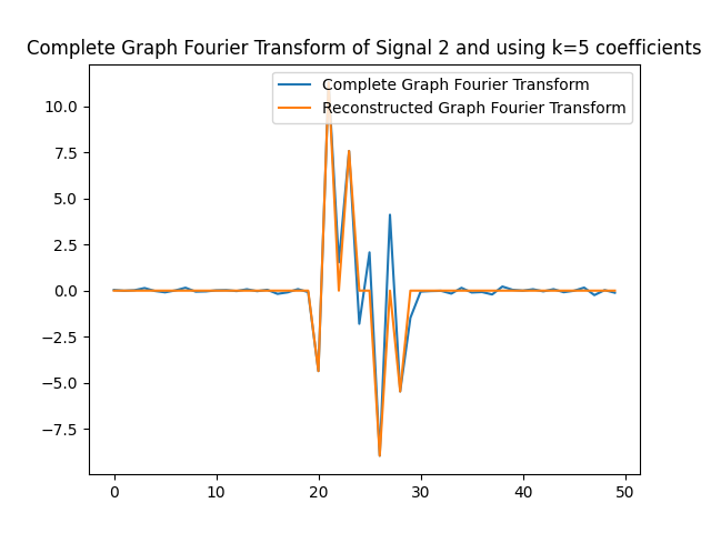
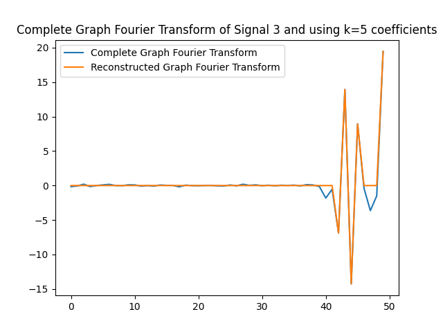
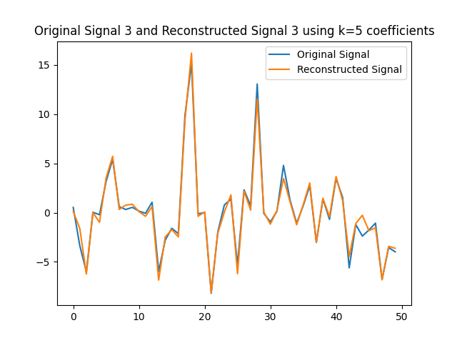
We can also assess how faithful to the original signal the reconstructed version is. Recall that in order to express the reconstructed signal using the $5$ coefficients with the largest absolute value, we are leveraging Parseval’s Theorem. In particular, the eigenvectors are othogonal, hence we can take the values of the coefficients. We can compute the reconstruction error which we express in the following table.
| Signal | Reconstruction error for $k=5$ |
|---|---|
| $x_1$ | 135.2 |
| $x_2$ | 181.5 |
| $x_3$ | 302.1 |
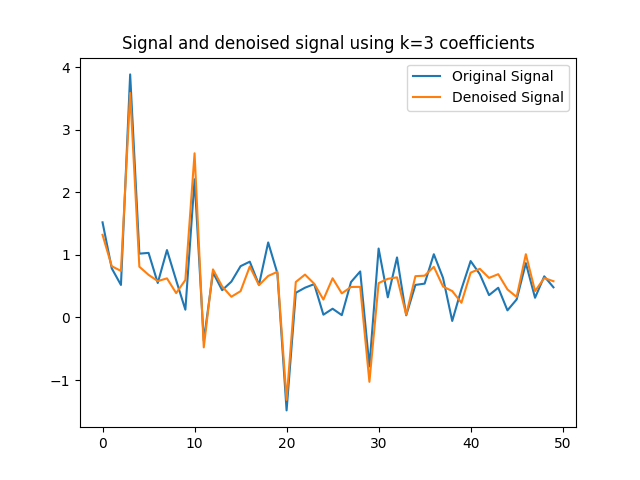
The last part of the homework asks us to compute a denoised version of graph signal $y$ using the largest $3$ components.
Code links
The code for this lab can be found here.