General MATLAB Functions
There are some MATLAB functions that, once coded in a given Lab, they will be used throughout the course. Here are these functions so everyone can have a unified version. This list will start growing as we progress through the Labs.
Obs.: In all cases execute help <name_of_function> before using them for the first time to understand how they work, their limitations and their syntax.
-
- cexp.m – Generate a discrete-time complex exponential.
- cexpt.m – Generate a continuous-time complex exponential.
- sqpulse.m – Generate a square pulse.
- tripulse.m – Generate a triangular pulse.
- dft.m – Compute DFT.
- idft.m – Compute iDFT.
- lpf_freq.m – Compute the LPF on a frequency spectrum.
- record_sound.m – Records a sound from your computer.
Installation
The idea is that these functions are set in such a way that they can be called from any directory where MATLAB is running. For this, be sure to save the functions in the following directories and restart MATLAB after downloading them.
-
-
- Linux: Download functions in directory /home/<username>/Documents/MATLAB
- Mac: Download functions in directory /Users/<username>/Documents/MATLAB
- Windows: Download function in directory C:\Users\<username>\MATLAB
-
Lab 1
Week 1, discrete sines, cosines, and complex exponentials (due on Friday 1/24). This lab is an introduction to three of the most important discrete signals we will be using in this course. We will investigate the behavior of complex exponentials with different frequency indexes and equivalent complex exponentials, and we will define orthonormality and its relation with the inner product discussed in class. Later, we will see how these concepts relate to the real world as we generate a musical note using a discrete cosine signal. Finally, we will use MATLAB to play “Happy Birthday.”
Or try these alternate songs generated by students in previous years:
-
-
- twinkle_twinkle.m – Twinkle Twinkle Little Star.
- ode_to_joy.m – Ode to Joy
-
Lab 2
Week 2, discrete Fourier transform (due on Friday 1/31). We have now seen the DFT expressed as abstract mathematical notation, but how can we implement this in the real world? In this lab, we will code a DFT function in MATLAB, and then use this to explore the DFTs of some signals we have seen in class (square pulse) and some that we have not (triangular pulse, Parzen windows, raised cosine, Gaussian, and Hamming windows). We will then prove some of the important properties of the DFT – conjugate symmetry, energy conservation (Parseval’s Theorem), and linearity, and conservation of inner products (Plancherel’s Theorem).
We will see some more applications of the DFT as it pertains to some real world signals that we are all familiar with – musical tones. By using the DFT, we will be able to investigate the spectra of an A note and the “Happy Birthday” song that we coded in the last lab. Finally, we will tie all this together to investigate the energy composition of “pure” note, as well as those that are characterized by harmonics – that is, “real” notes of various instruments.
Lab 3
Week 3, inverse discrete Fourier transform (due on Friday 2/7). The iDFT is, as you might expect, the inverse operation to the DFT. After proving why this is true, we will see some of its uses in signal compression and reconstruction. We will see that we can get a pretty good approximation of a signal by storing only a few of its frequency components. This should prompt some questions. Why can we do this? Which components should we store? We will look at the energy of the error signal (the difference between the original and reconstructed signals), which will give us a hint. We will explore these topics further in later labs.
Next, we will take these techniques of compression and reconstruction into the practical domain. We will record an audio signal (a voice recording), and look at how the DFT and iDFT can be used to manipulate this signal. We will see that the complexity of this signal makes this a difficult task. What would happen if we divided the signal into sections and applied these techniques to each section? (Hint: this is what a primitive MP3 compressor and player does). For extra credit, we will try to use signal processing to decode a secret message.
Secret Message
-
-
- x.mat – Here is the scrambled voice signal for Part 3.
-
Lab 4
Week 4, Fourier transform (due on Friday 2/14). We will take a break from the more computational labs and take a look at a purely analytical tool – the Fourier transform. We will compute a few useful Fourier transforms, namely that of a Gaussian pulse. Perhaps most importantly, we will see how the DFT serves as an approximation to the Fourier Transform.
Next, we will investigate the modulation and demodulation properties of the Fourier transform, which are much easier to see here than with the DFT. We will learn what a bandlimited signal is and why it is useful if we want to modulate. We will use these properties to modulate a voice recording, and then we will use these same properties to “decode” and recover the original recording.
Lab 5
Week 5, sampling (due on Friday 2/21). What happens when we sample a signal to process it in a computer? This is one of the foundational questions of this course, and we will investigate it in depth in this week’s lab.
We will see how we can use Dirac trains to mathematically represent sampling. Next, we will see why bandlimited signals prevent information loss when sampling, and what information is lost when a signal is not bandlimited. We will see that, while Dirac trains do not exist in reality, they can be approximated with tall, narrow pulses. We will derive just how tall and narrow these pulses need to be.
Finally, we will investigate subsampling. We will see many of the properties discussed in lecture in action. Specifically, we will note two key relationships:
-
-
- Sampling in time leads to periodization in frequency.
- Filtering reduces aliasing (information loss).
-
Lab 6
Week 6, voice recognition (due on Friday 2/28). There will be no new concepts introduced in this lab. Rather, we will integrate all of the knowledge of signal processing that we’ve learned thus far to create a voice recognition system. We will learn how to use training sets and test sets, along with a comparison algorithm (in this case nearest neighbor), to identify an unknown spectrum. This will allow us to distinguish between the spoken digits “one” and “two.”
For extra credit, we will extend this system to recognize the spoken digits zero through nine. We will see that this is more difficult, and we will use our knowledge of the frequency domain to reason why.
Lab 7
Week 7, voice recognition with a filter (due on Friday, 3/6). This lab is very short, and is just an extension of Lab 6. We know that multiplication in frequency is equivalent to convolution in time, but how does this help us? We will see that we can take the voice recognition algorithm from Lab 6 and apply it in “real time” – that is, it will be able to detect a continuously spoken sequence of digits.
This would be difficult to do in frequency, so we will use the design of Lab 6 that we created in the frequency domain and implement it now in the time domain via the convolution. Cool!
Lab 8
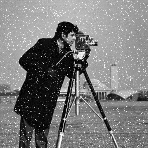
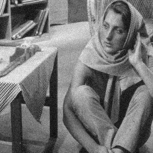
Week 8, image processing part 1 (due on Friday, 3/27). In this lab, we will repeat pieces of previous labs with one key difference: we are now working in two dimensions instead of one! We will revisit the concepts of orthogonality, energy, square and Gaussian pulses, DFTs, and iDFTs with this new frame of reference.
We will then see this results in action in as we de-noise an image by filtering with a Gaussian pulse. This visual application of signal processing is a direct extension of what we’ve learned in the first half of the course!
Images for Lab: Image A Image B
Lab 9
Week 9, image processing part 2 (due on Friday, 4/3). This lab well reinforce the key concepts of image processing that we saw in Lab 8. However, we have seen that the 2D DFT can have some undesirable border effects. We will fix this with the discrete cosine transform (DCT).
We will investigate compression and reconstruction with the DCT, and compare our results to those of the DFT. We will also introduce the concept of quantization as it relates to images, which is how rudimentary JPEG compression works!
Images for Lab: Image A (pre-noise) Image B (pre-noise)
Lab 10
Week 10, principal component analysis (PCA) part 1 (due on Friday, 4/10). This lab will introduce the technique of principal component analysis (PCA). We well see how essential information about a data set is contained in its covariance matrix, and we will use the eigenvectors of this matrix to “transform” our signal to the PCA domain. This is analogous to the frequency domain for a time signal!
We will reconstruct a given face using a varying number of principal components, and we will examine the reconstruction error to quantitively show us our accuracy. How should this accuracy compare to the DFT?
Lab 11
Week 11, face recognition, principal component analysis (PCA) part 2 (due on Friday, 4/17). In this lab we will apply the concept of PCA learned from the previous lab to construct a face recognition algorithm. We will see how the PCA transform captures the essential stochastic information contained in the faces in just a few values – far less than with the DFT – and, thus, allows for very efficient classification.
Lab 12
Week 12, graph signal processing (due on Friday, 4/24). In our penultimate lab, we will continue our trend of abstractions to introduce graph signal processing. Graph signal processing is an even more abstract way to define a signal over a graph, a category under which everything we have already covered falls. We will learn the basics of graph theory, and then apply these concepts to examine the frequency representation of a graph signal, including quantifying variations, reconstruction and Parseval’s theorem, and denoising.
This is an active area of research, and there is still much to be discovered about graph signal processing!
Lab 13
Week 13, classification of cancer types (due on Friday, 5/01). In this final lab, we will use our knowledge of graph signal processing for the particular application of identifying and classifying cancer types, which is a signal defined on a graph of gene networks. We will use the fundamental concepts of signal and noise, low and high “frequencies,” and filters to do so.